Baseline Transformer
Every experiment needs a good baseline. For this little Language Model (lLM) series, the baseline performance will be based off a standard transformer. A transformer is a model consisting of attention layers that adjust each token embedding via an all-to-all mechanism that both decides the degree of influence each token should have over each other token, and how that influence should modify each token. Many in-depth descriptions of transformers exist (e.g. this video and this blog post.) so I won’t rehash that, however I will say that I believe the key mechanism that makes transformers powerful is that, unlike models like convolutional neural networks (CNNs) which hard-code nearest neighbour interaction structure or dense neural networks (DNNs) which assume all features have equal impact on all other features, the effective learnability of the interaction structure allows transformers to more efficiently utilise information. They are extremely efficient to train, using each token in a sequence as an example effectively boosts the batch size by an order of magnitude.
Optimising Hyperparameters
I don’t think it’s a particularly controversial statement that the least fun part of training models is hyperparameter optimisation. I want to minimise the amount that I do this, so this section develops an automated process that tunes the depth of the model and the learning rate. This process is intended to be reused across experiments. While optimum hyperparameters don’t necessarily transfer between architectures, I make the assumption that using the majority of hyperparameters tuned for the transformer model will give good enough results for comparison in this context. Additionally, since the transformer is so well-established, any disruptor model will have to outperform it by a non-trivial amount, in which case this would likely account for the sub-optimally tuned hyperparameters. That being said, the learning rate will be optimised for all experiments, and the largest batch size possible on the gpu will be automatically detected.
The three parameters I optimised for are the learning rate scheduler, the tokens per parameter used to train the model, and the vocabulary size. All other hyperparameters used feasible values typical of models trained on this budget.
Learning Rate
Firstly, I investigated the learning rate optimisation process to produce the best results. For these experiments, the token count was set to the chinchilla-optimal 20 tokens per parameter and the vocab size was set to 4K, a value used by a few papers training on BabyLM. I chose to use OneCycleLR as the scheduler, and ran a learning rate sweep over three parameter configurations: one relatively standard OneCycle with the peak 30% through the entire training run, with the initial learning rate divided by 3 and final divided by 10, one aggressive schedule where the peak happens 5% the way through the run, with the initial and final learning rates divided by 10 and 100 respectively, and one medium approach with the peak at 10% and division factors of 6 and 20. The results are shown in the following graph: 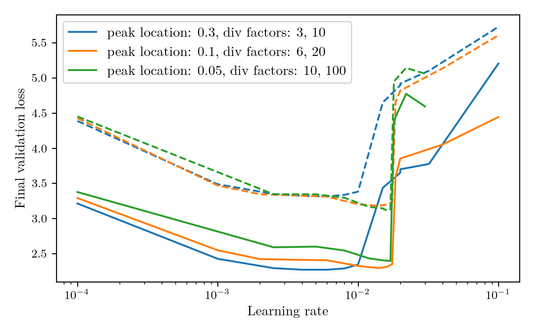 Where the solid line is the final training loss and the dashed line is the validation loss. All three show a similar behaviour of a gradual decrease and low plateau, followed by a sharp increase in the loss where the training has become unstable. The medium approach achieved the lowest validation loss, while also maintaining the smallest gap between train and validation performance, so this was the method chosen.
To optimise the learning rate for a model, a reasonable method is to run the training for the first x% of steps, and then continue with the option that achieved the best validation loss. However, early performance is not always indicative of final performance and can often indicate an overly high learning rate that finds a poor minimum early on. To investigate the robustness of the early stopping method of tuning the learning rate, I used the learning rate sweep data to calculate the correlation between the validation loss at each step and the final validation loss. If this is high, it gives confidence that a low validation loss at that point will obtain a good final model, while a low correlation would indicate that it is a not a reliable signal. The correlation as a function of step number can be seen below. 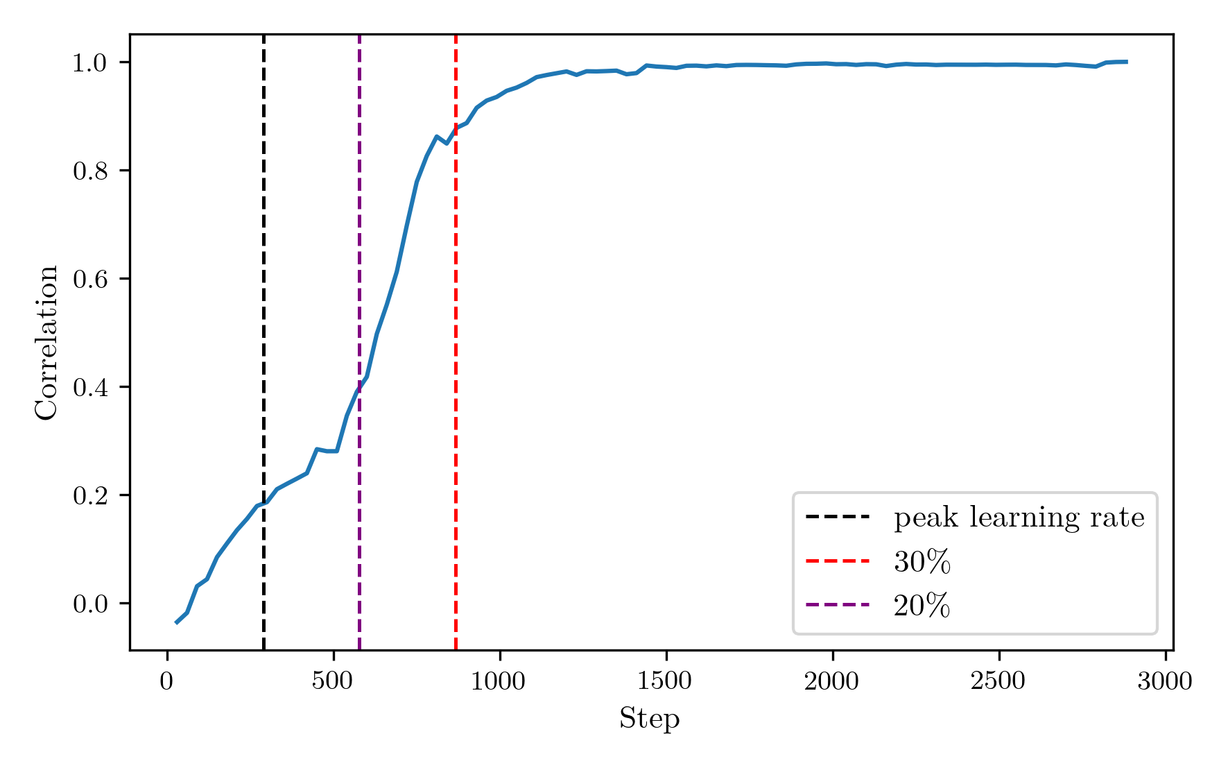 As expected, the loss at the very first step has essentially no correlation with the final outcome, while by definition the final step has perfect correlation. The correlation increases over the first 30% of the training steps, then plateaus for the rest of the run. Therefore, 30% would be an ideal time to choose the final learning rate. However, 30% of the full training course is a rather expensive optimisation procedure, and testing a few learning rates would lead to this step taking longer than the full training run, time which could potentially be better spent in actual training. Therefore, I am going to choose to determine the learning rate at 20% of the run. While the correlation is significantly weaker here, it allows for five learning rates to be measured in the training budget, and the shallow plateau of the loss curves indicate that the loss is likely to be good enough. Applying this rule to the peak location: 0.1, div factors: 6, 20 learning rate sweep from before, the final learning rate chosen would have been 0.012, obtaining a near optimal final validation loss of 3.16. This learning rate is displayed in the following plot by the vertical line superimposed on the learning rate sweep from earlier.
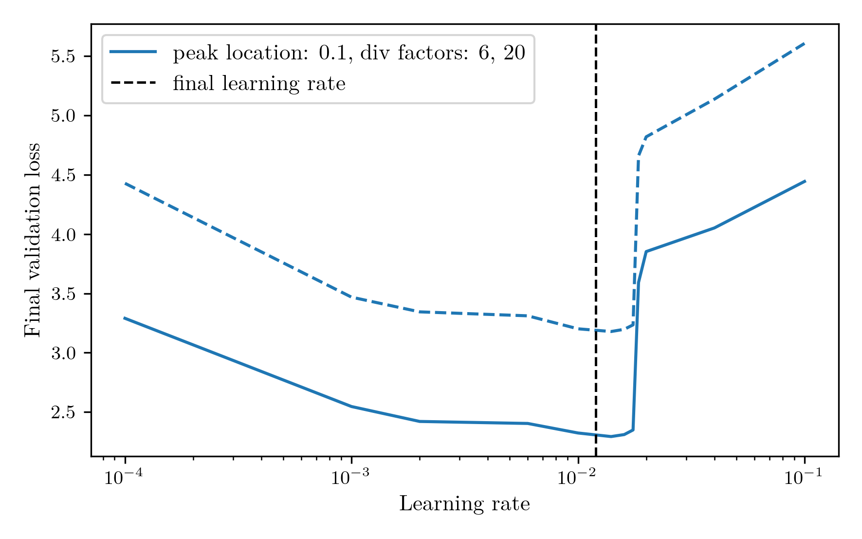
Vocab Size
Now that the learning rate optimisation process has been decided, it’s time to choose the vocabulary size. For this, I kept the tokens per parameter at 20 and slotted in the learning rate optimisation process. I trained unigram tokenizers on 10000000 rows of BabyLM with vocabulary sizes of 1K, 2K, 3K, 4K, 6K, 8K, 10K, 12K, 15K, and 20K. I then ran training experiments with each vocabulary size. Unfortunately, validation cross-entropy loss is not directly comparable between different vocabulary sizes because an increased vocabulary size increases the total amount of possible entropy, and additional tokens end up being longer on average, resulting in a decreased number of tokens over the whole validation set. To account for this, these results are compared using bits per byte (BPB), which is computed using the average bits per token over the validation set for each vocab size. The results are as follows. 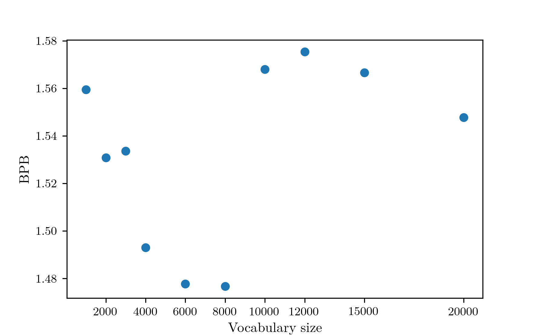 The performance decreases from the early vocab sizes to reach a minimum at around 8K, which is the vocabulary size that will be used from here on out. There is an outlier at 3K, which likely stems from the fact that I am only performing a single run for each vocab size. There is also noise after 10K, which could stem from the same thing. However, I noticed in these runs that the learning rate chosen was the smallest of the set, so from now on the learning rate lower bound will be decreased to 1e-4. So far, all the tests have been performed with vocabularies created via the unigram method. I ran one test for a BPE tokenizer with vocabulary size 8K, and it achieved a validation BPB almost identical to the the unigram tokenizer. Since it doesn’t seem to affect the results that much, I’ll choose the unigram tokenizer. For future experiments with different architectures, the vocabulary size is probably better fixed as a ratio between the number of parameters in the encoding and the number in the rest of the model, but to do that would require more complex pretraining, more tokenizer options, and more complicated metrics, so the vocabulary size will be fixed at 8K for all future experiments.
Tokens per parameter
One of the major milestones of recent AI research was the chinchilla series of experiments, in which they demonstrated the existence of scaling laws that persist over many orders of magnitude of model sizes. One parameter for which such a scaling law exists is the ratio of tokens to parameter used to train a model given a fixed compute budget. They found it to be around 20, which is the value I have been using for the tests so far. The current logic finds the largest model that can throughput at least 20 tokens per parameter in the 30 minute training window. For the 8K vocab run from before, that resulted in a 21 layer model. I ran a sweep of the model size to investigate the performance of different tokens per parameter values. The tokens per parameter obtained by different layer sizes is as follows. 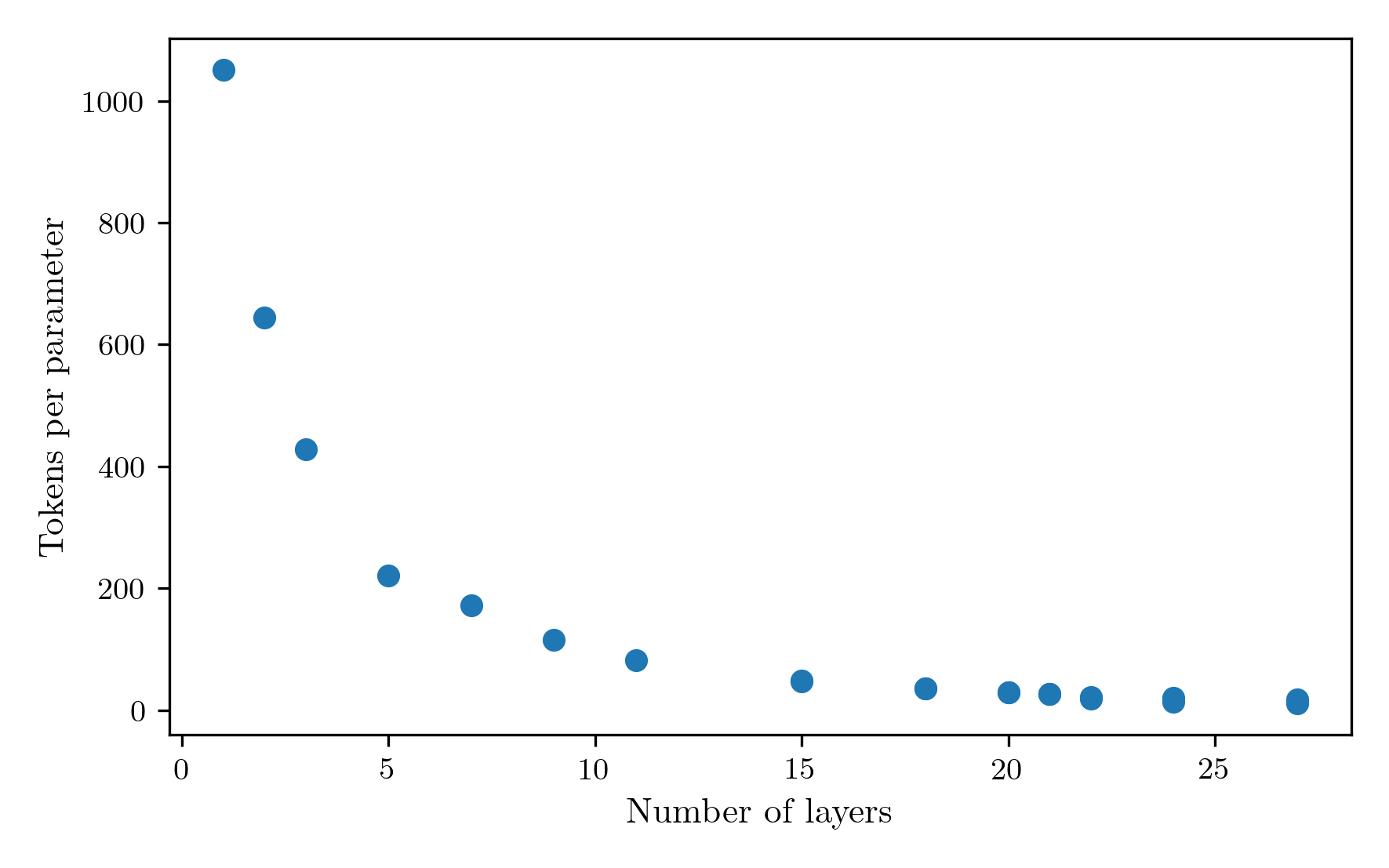 Reducing the number of layers both decreases the number of parameters, and increases the token throughput as a result of reduced computation. The result is a 1/layer_count scaling of tokens per parameter. The performance of the model at different token counts is shown in the next figure.
 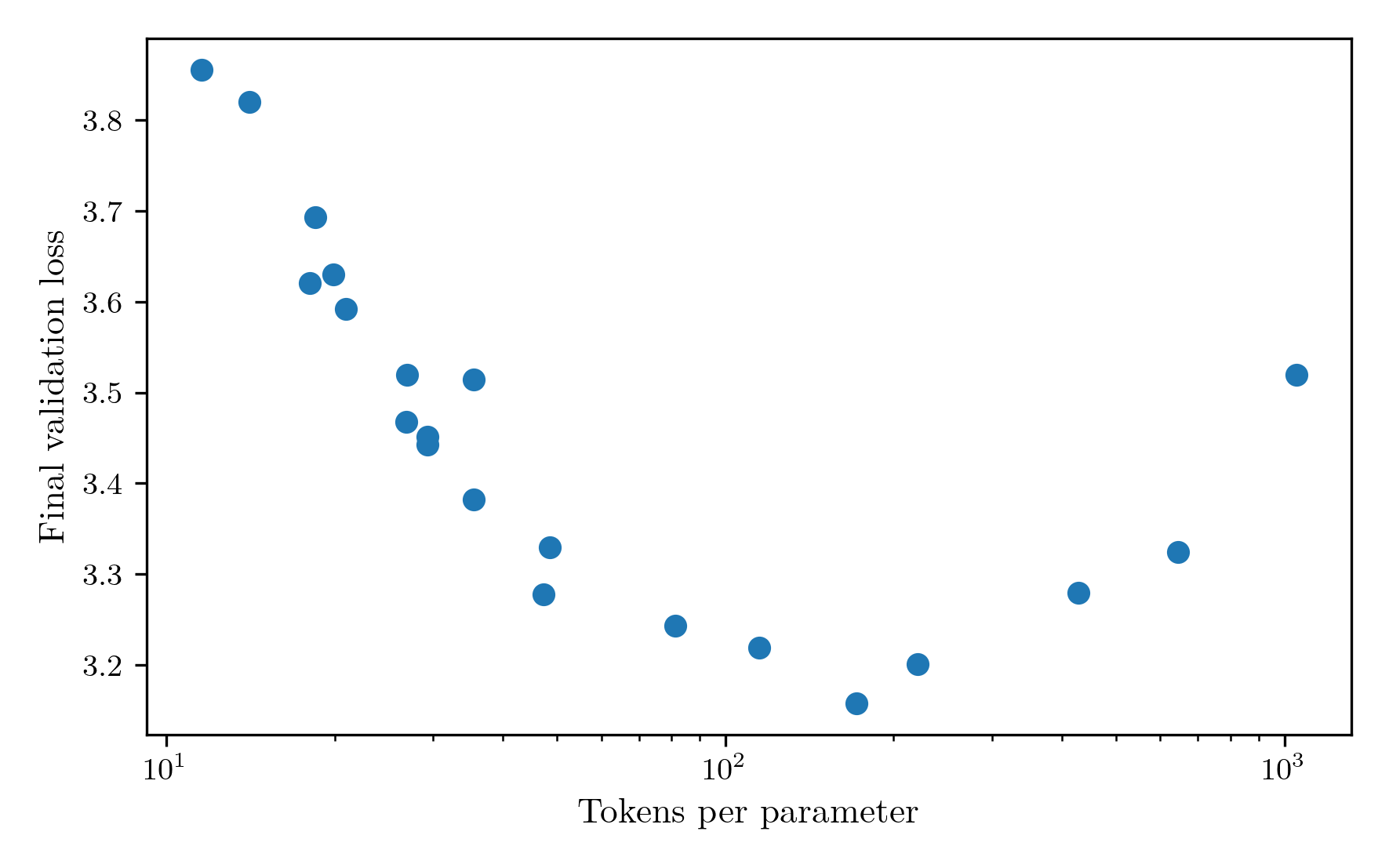 The most performant model occured at a layer count of 7, achieving 171.6 tokens per parameter. I found this result very surprising. It is far away from the chinchilla optimal result, has a high fraction of its parameters contained in the embeddings only, and my intuition was telling me more depth would be needed for a good result. I can think of three reasons that could be causing this to happen.
Firstly, this could just be the optimal number of tokens per parameter for this set up. The chinchilla experiments only went down to models with about 100M parameters, while a 21-layer model in this set up has only 18.5M parameters. It could just be that in this regime, with this dataset the token requirements are a lot higher.
Secondly, because the format of the dataset introduces a new row for every single line of text, including different utterances of a conversation, I have been creating an IterableDataset where neighbouring rows are merged together as a sequence prior to batching. While this has some local shuffling via a buffer, the data does appear on average in order. In contrast to this, the validation set is constructed from samples interspersed through the whole dataset. Therefore, an increase in tokens per parameter could mean that more of the entire dataset is seen, so while it may not perform as well on examples that it has seen, on average the validation loss improves.
Finally, and I think most likely, is that the accumulated batch size is horribly misconfigured. With the limitation of 30 minutes of training, there are only so many gradient steps that can be performed. That could mean that if the batch size is too high, there simply aren’t enough gradient steps to travel from the initialised parameters to a good minimum, and the high tokens per parameter value is prioritising obtaining more descent steps above all else. To investigate this, I ran a sweep of the accumulated batch size, keeping tokens per parameter at the chinchilla value of 20 for now and using the same learning rate sweep as before. The batch size sweep confirmed my suspicions that the batch size was far to big, with the minimum loss occurring at 51. 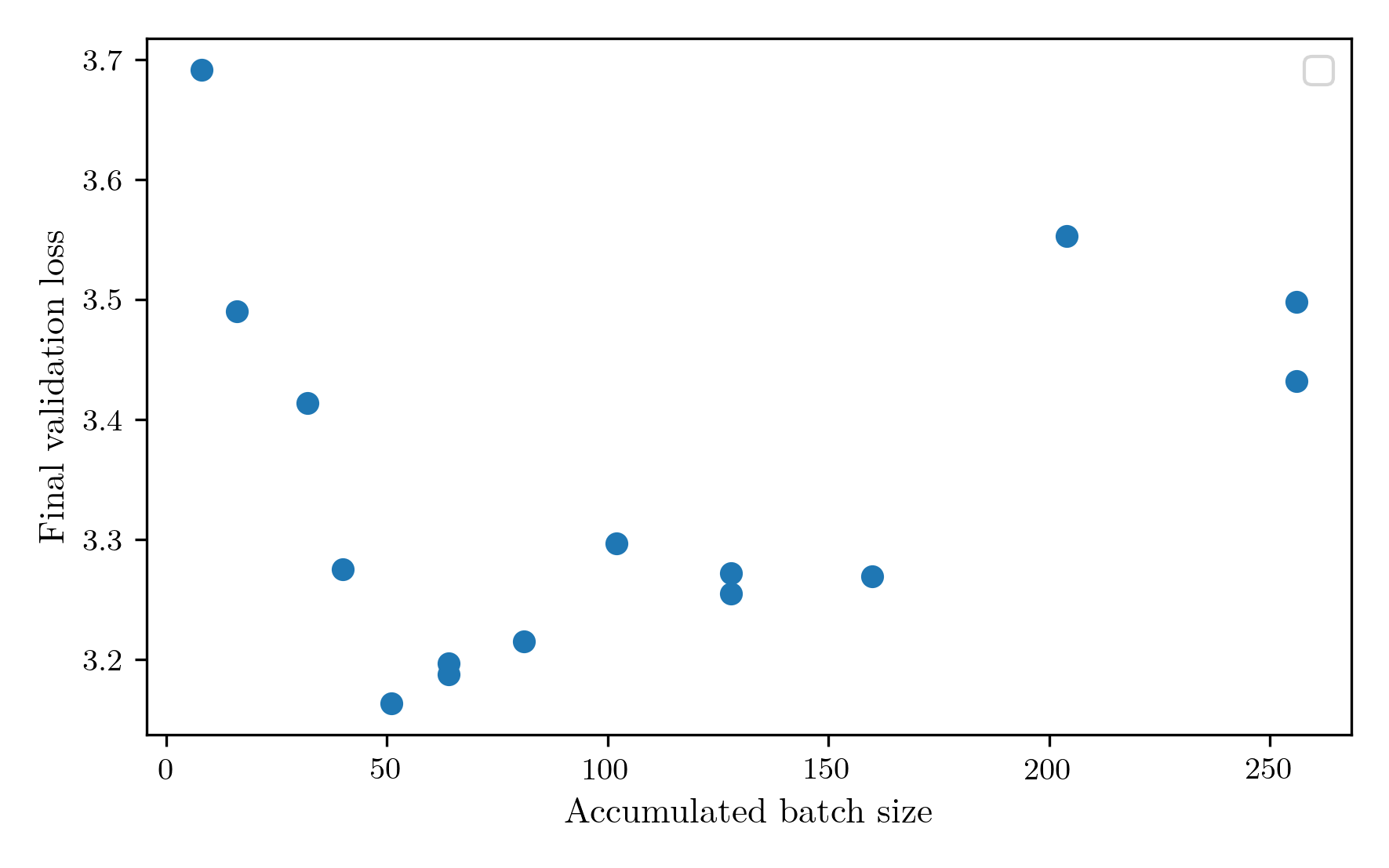 Rerunning the tokens per parameter sweep, the optimum falls around 70, much closer to the chinchilla expectation.
At about this point, I’ve realised that my original intention to save time and money by manually optimising the hyperparameters was a gross miscalculation, and I have actually spent much more time and money doing this than setting up a big optuna run to find the best hyperparameters algorithmically. Also, my manual single-variable sweeps can’t find dependencies between hyperparameters, which are probably significant, for example between vocab size and tokens per parameter. Since I also want to train these models on the simplestories dataset, I decided to just bite the bullet and spend 10 hours each on training 100 6-minute tests for models on each dataset. It seems a bit silly spending 10 hours tuning the hyperparameters for a 30 minute training procedure, but the intention is to not adjust these hyperparameters across future architecture changes, so it’ll help if they’re pretty good. It allowed me to also investigate the width of the models by varying the embedding dimension and number of attention heads. The resulting distribution of parameters obtained showed sensible properties, with most having a smooth minimum somewhere in the range. The key exception was the layer number parameter for the BabyLM dataset, which displayed an inverted parabola shape, indicating a bimodal distribution that can perform well at small layer counts or larger layer counts, presumably dependent on one of the other parameters. 
The final Optuna-identified parameters for the models are as follows:
| Dataset |
Layer Count |
Accumulated Batch Size |
Learning Rate |
Embedding Dim |
Attention Heads |
Vocab Size |
| BabyLM |
32 |
32 |
0.014664 |
192 |
6 |
12000 |
| SimpleStories |
5 |
64 |
0.006036 |
288 |
3 |
8000 |
The model for babylm massively prefers increased depth and complexity via its attention heads and vocab size, whereas the SimpleStories prefers a shallow, wide model with more examples processed. This makes sense as the SimpleStories dataset is designed to use minimal, simple vocabulary and simpler grammatical constructions, while the BabyLM dataset is not restricted in its grammar or content.
To evaluate the parameters, I trained two models with each set of hyperparameters (BabyLM-optuna, BabyLM-manual, and SimpleStories-optuna) and averaged the BPB.
| Model |
Bits per Byte |
| BabyLM-optuna |
1.45 |
| BabyLM-manual |
1.33 |
| SimpleStories-optuna |
0.57 |
Interestingly, the manual search for BabyLM achieves a better final BPB than the optuna search after all. It’s reassuring to be reminded of the continued effectiveness of grad student descent. The failure of optuna here could stem from a breakdown of the correlation between 6-minute validation loss and 30-minute validation loss at this wider hyperparameter range, or the fact that BPB is calculated using the average bits per token over the whole training set while the optuna run is validated on only 30 batches. Either way, the manually identified hyperparameters perform better, so those are the ones I’ll use. This also implies that SimpleStories could benefit from some manual tuning, but the time, money, and patience budget for hyperparameter tuning are thoroughly exhausted for this project, so we’ll stick with what we’ve got.
Full training process
The final training process is then as follows. The model and data parameters are selected from the hyperparameters found from this experiment process for each dataset. During the training run, the number of layers is swept until the tokens per parameter target of 70 for BabyLM and 175 for SimpleStories is achieved. During the layer sweep, the batch size for good utilisation of the GPU is also found. Then, five 6-minute runs are tested to compute the optimum learning rate for the architecture at hand. Finally, the model is trained for 30 minutes and the results stored.
The commits to access the final training runs are here:
BabyLM-manual:
Example generations:
caitlin stood on the edge of the cliff.
jayden had a jolly good time, and he was a good swimmer.”
in japanese culture, women are often used to be used to make a living.
SimpleStories:
Example generations:
caitlin stood on the edge of a cliff. below, a small village lay quiet, with only the sound of waves crashing. a boy named leo stood at the edge, staring into the dark water. he had heard tales of a lost city beneath the waves, a place where dreams came true. with a deep breath, he jumped into the water. the cold water wrapped around him like a blanket, and he swam deeper. as he swam, he saw strange shapes in the shadows. they looked like fish, but they
jayden had a jolly good time. a girl named alice loved to bake cookies. one day, she decided to bake a cake for her friends. she wanted to make the best cookies ever. but when she mixed the batter, she forgot to add sugar. “oh no!” she cried. she looked at the mess and felt sad. then, she remembered her mom's advice: “don't worry, i can fix this!” she took a deep breath and started to work. she mixed the batter and added chocolate chips
in japanese culture, women are often seen as they celebrate the harvest festival. they wear bright clothes and dance, celebrating the harvest. among them was a young woman named mia. she was known for her beautiful clothes and her beautiful clothes. but she felt a little lost. she wanted to be part of the festival, but she was afraid. one day, while walking through the market, mia saw a man selling fruits. he was selling fruits and spices. she felt a spark of hope. “i can buy these,” she thought
]]> And the BPB results show a loss minimum at projection dim 96.
 However, the unprojected baseline outperforms all projected experiments.
Intuitively, this would indicate that the expressivity is saturated, but then I wouldn’t expect to see the minimum at 96.
To get to the bottom of this, I investigated the total tokens processed by each model.
However, the unprojected baseline outperforms all projected experiments.
Intuitively, this would indicate that the expressivity is saturated, but then I wouldn’t expect to see the minimum at 96.
To get to the bottom of this, I investigated the total tokens processed by each model.
 The token counts are all over the place, not the smooth decrease I’d expect as projection_dim is increased.
The dense baseline actually achieved the highest token count of all.
Maybe the total descent steps calculation is inaccurate and some are getting more time?
Here is the plot of the tokens processed per second, which shows that while some may have gotten more total time, the actual rates are more noise than signal.
The token counts are all over the place, not the smooth decrease I’d expect as projection_dim is increased.
The dense baseline actually achieved the highest token count of all.
Maybe the total descent steps calculation is inaccurate and some are getting more time?
Here is the plot of the tokens processed per second, which shows that while some may have gotten more total time, the actual rates are more noise than signal.
 I’m not sure there’s much that can be gleaned from this data except that latent attention does not help performance on a small restricted training budget, at least with this set up.
One thing that can be investigated is compilation.
With these small dimensions, the overhead of matmul kernel launches on the GPU may be affecting performance significantly.
Fortunately, PyTorch provides a JIT compiler to try to mitigate these issues.
I tested compiled versions of the baseline unprojected model and a latent attention model, each with three seeds.
I’m not sure there’s much that can be gleaned from this data except that latent attention does not help performance on a small restricted training budget, at least with this set up.
One thing that can be investigated is compilation.
With these small dimensions, the overhead of matmul kernel launches on the GPU may be affecting performance significantly.
Fortunately, PyTorch provides a JIT compiler to try to mitigate these issues.
I tested compiled versions of the baseline unprojected model and a latent attention model, each with three seeds.
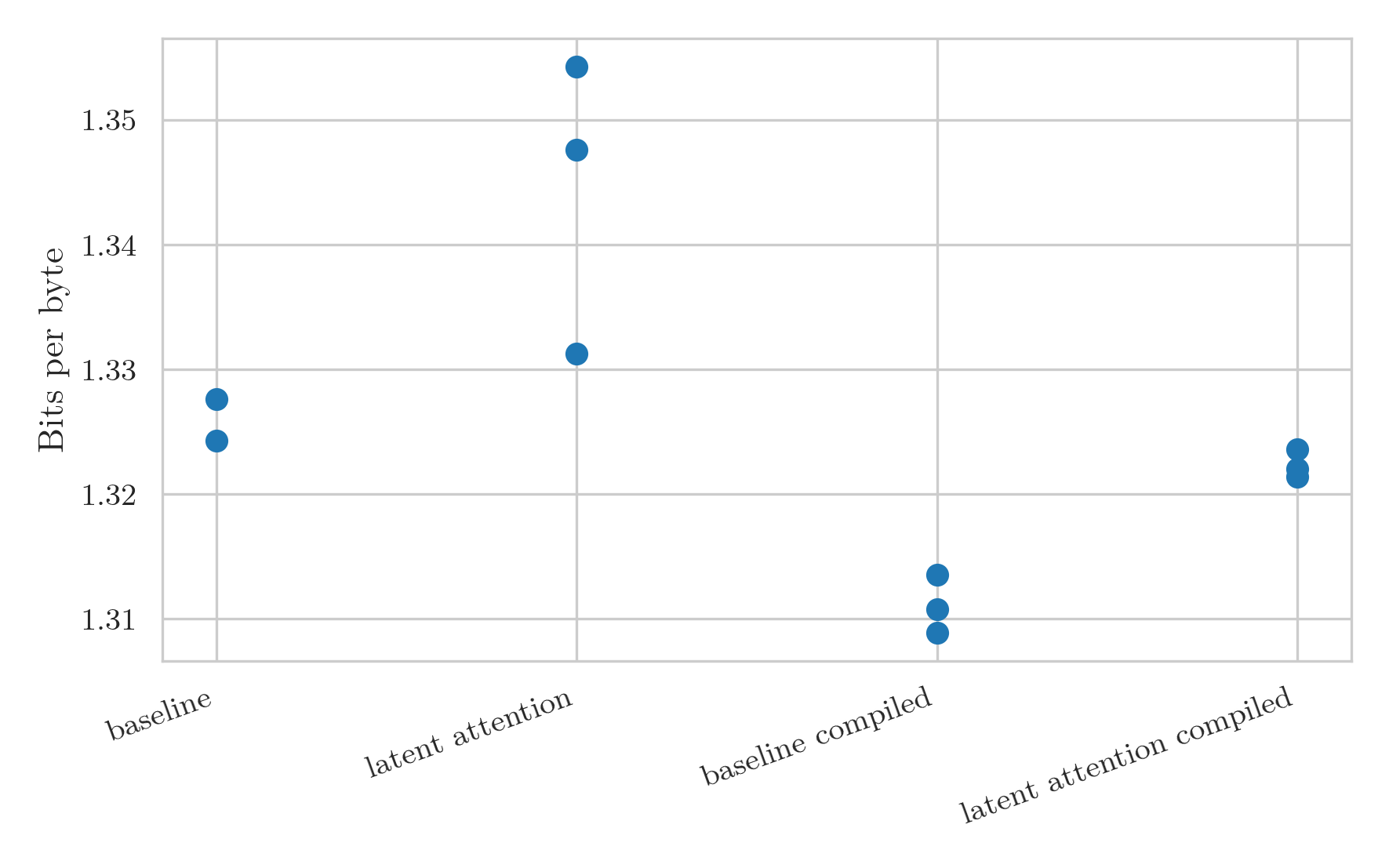
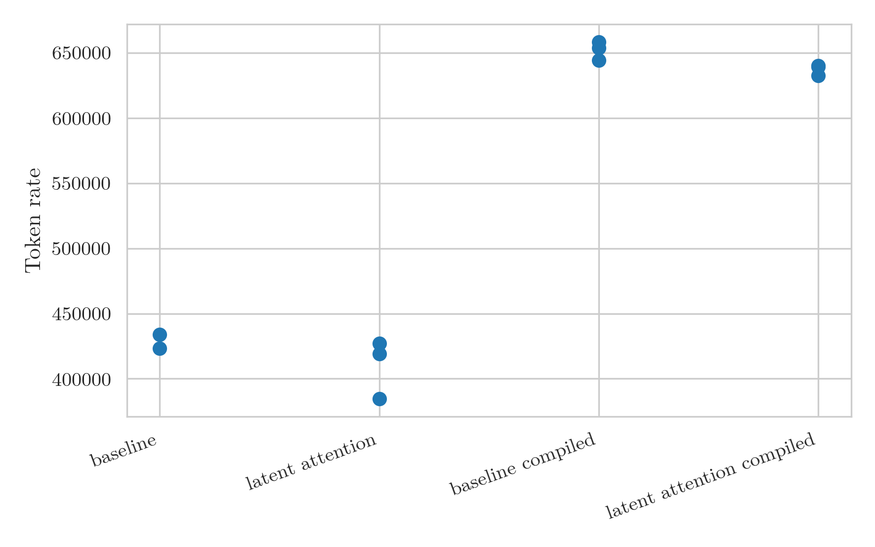 This was a great success. Not only is the throughput massively higher, but it is also much less noisy.
The increase in token rate leads to a distinct decrease in the BPB for the models:
This was a great success. Not only is the throughput massively higher, but it is also much less noisy.
The increase in token rate leads to a distinct decrease in the BPB for the models:
 The main problem with the compiled version is that the probes that calculate how many descent steps fit in 30 minutes are thrown off by the initial compilation.
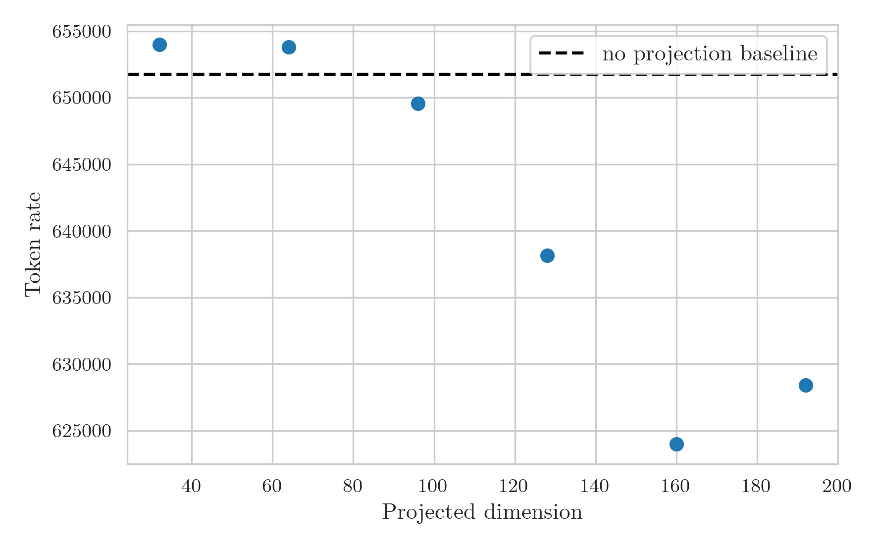
I ran the projection sweep again, and adjusted the warmup steps to 200 and memory test steps to 100 to attempt to account for the compilation time.
While the runs still didn’t go for the full anticipated 30 minutes, taking around 26 minutes instead, the results make a lot more sense than the previous graphs.
The token rate graph now shows a smooth decrease in rate as projection dimension increases, with a high bar from the baseline model likely stemming from the GPU overhead arising splitting the KV multiplication into two separate multiplications.
The main problem with the compiled version is that the probes that calculate how many descent steps fit in 30 minutes are thrown off by the initial compilation.
I ran the projection sweep again, and adjusted the warmup steps to 200 and memory test steps to 100 to attempt to account for the compilation time.
While the runs still didn’t go for the full anticipated 30 minutes, taking around 26 minutes instead, the results make a lot more sense than the previous graphs.
The token rate graph now shows a smooth decrease in rate as projection dimension increases, with a high bar from the baseline model likely stemming from the GPU overhead arising splitting the KV multiplication into two separate multiplications.
 The BPB graph is still a bit noisy at large projection dimensions:
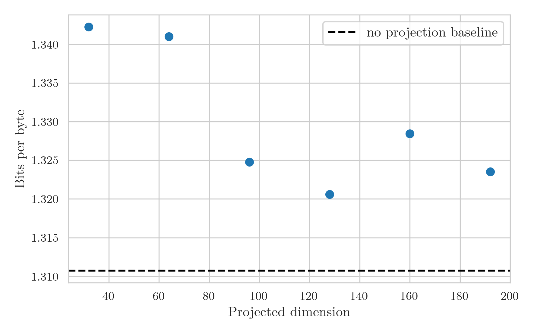 But I think shows a couple of things quite clearly.
Firstly, the expected pattern is now seen.
The BPB decreases as projection dimension increases due to the increased expressivity of the layer.
However, at a dimension of around 128, a minimum is achieved where above this the added cost restricts the number of tokens processed enough that the model starts to perform worse.
Secondly, the overhead from breaking up the matrix multiplication drowns out any performance gain from reduced FLOP and parameter counts, at least at this small scale.
This means that latent attention likely isn’t a viable method for increasing training performance, and should be used for its primary use case of increased KV caching efficiency.
But I think shows a couple of things quite clearly.
Firstly, the expected pattern is now seen.
The BPB decreases as projection dimension increases due to the increased expressivity of the layer.
However, at a dimension of around 128, a minimum is achieved where above this the added cost restricts the number of tokens processed enough that the model starts to perform worse.
Secondly, the overhead from breaking up the matrix multiplication drowns out any performance gain from reduced FLOP and parameter counts, at least at this small scale.
This means that latent attention likely isn’t a viable method for increasing training performance, and should be used for its primary use case of increased KV caching efficiency.