Latent Attention
One of the key innovations DeepSeek made when they disrupted the LLM space was the introduction of latent attention. Latent attention decreases the parameter overhead of the attention mechanism by splitting it into two parts. The first part takes the embedding vector and reduces it to a vector of lower dimension via a rectangular matrix. The second part then reprojects this intermediate latent vector into the K and V vectors needed for attention. This process reduces the parameter count of attention as a single matrix of shape [embedding_dim, KV_dim] uses significantly more parameters than two matrices of [embedding_dim, projection_dim] and [projection_dim, KV_dim] for a sufficiently small projection_dim. Not only that, but DeepSeek actually shares the first half of the layer over all K and V vectors. This both reduces the parameter count further, and allows the compressed latent KV vectors to be cached with reduced memory cost, at the cost of reprojecting them each time. The latent intermediate vector design exploits the low-rank nature of attention. Since each attention head focusses on a subset of the properties of each embedded token, these properties likely have a lower effective dimension than the full embedding space. Explicitly building this assumption into the model results in a decomposition similar to a Singular Value Decomposition (SVD), where a matrix is decomposed into two orthogonal matrices and a diagonal matrix containing the singular values, revealing the rank structure of the original matrix. By absorbing the singular values into either of the orthogonal matrices, a split two-step approach pops out, exactly as previously described. The two-stage construction of latent attention is not strictly comparable to an SVD since the rectangular matrices are not constrained to be orthogonal. However, it does constrain the rank of the combined transformation the same way as performing an SVD and truncating the singular values would.
While I think that the primary concern for the DeepSeek researchers was the inference efficiency and therefore the effectiveness of the KV caching, for a fixed training compute budget I am interested to find out if the increased parameter efficiency results in models that perform better than full-rank attention. My prediction is that BabyLM will benefit from latent attention, as it will allow an increase in the depth of the model for the same parameter count.
Implementation
The implementation of latent attention is very simple. In my repository, I simply override the KV transformation with the latent version:
self.kv = nn.Sequential(nn.Linear(embedding_dim, projection_dim),
                        nn.Linear(projection_dim, (self.qk_dim + v_dim) * n_heads))
It seems that the standard implementation uses a latent representation for K and V, but not Q. This is likely due to the main intention being for caching efficiency, since Q is not typically cached. In our case, where we are investigating if reducing parameter count can increase performance on a fixed training budget, it may be worthwhlie to also compress Q. However, the degree of precision needed to adequately describe the query is likely greater than the target. For each attention call, each query is compared to many keys and values, so precision of the query is likely more important than that of the keys and values. Based on absolutely nothing but this unsubstantiated hand-wavy argument and the fact that DeepSeek didn’t do it, I will not compress Q.
Projection dim sweep
I decided to sweep the projection dimension on the BabyLM dataset. The embedding dimension is 256, the qk dimension is 64, with 4 heads and the matrix is shared between both k and v, so the full final dimension is 512. A full-rank matrix would use 256 * 512 = 131072 parameters, and a projection dim that matches this would use (256 * p_dim) + (512 * p_dim) = 131072 -> p_dim = 170.6, so the projection dim has to be smaller than that in order to save parameters. We can calculate the same thing for FLOPs. Assuming naive matmul, the cost of the unprojected attention is batch_dim * seq_dim * 256 * 512, and the latent version is batch_dim * seq_dim * 256 * p_dim + batch_dim * seq_dim * pdim * 512. Dividing through by the batch and sequence dimensions, we arrive at the same crossover point for FLOPs The sweep tests values 16, 32, 48, 64, 80, 96, 112, 128, 192, and 256. These tests gave quite noisy results, so I ran each twice and averaged the results. I would expect projected dimension 171 to achieve approximately the same performance as the dense model since it uses the same number of parameters and compute. I would also guess that decreasing the projection dimension could improve the performance, as the reduced cost would allow more tokens to be processed. At some point, the expressivity of the reduced projection dimension will get so low that the performance will get worse again. Another scenario that could occur is if the expressivity of the dense attention is already saturated, the latent attention will perform strictly worse.
The sweep gave me very confusing results.
Firstly, the parameter count graph follows the predicted pattern, with the crossover at 171.
 And the BPB results show a loss minimum at projection dim 96.
 However, the unprojected baseline outperforms all projected experiments.
Intuitively, this would indicate that the expressivity is saturated, but then I wouldn’t expect to see the minimum at 96.
To get to the bottom of this, I investigated the total tokens processed by each model.
However, the unprojected baseline outperforms all projected experiments.
Intuitively, this would indicate that the expressivity is saturated, but then I wouldn’t expect to see the minimum at 96.
To get to the bottom of this, I investigated the total tokens processed by each model.
 The token counts are all over the place, not the smooth decrease I’d expect as projection_dim is increased.
The dense baseline actually achieved the highest token count of all.
Maybe the total descent steps calculation is inaccurate and some are getting more time?
Here is the plot of the tokens processed per second, which shows that while some may have gotten more total time, the actual rates are more noise than signal.
The token counts are all over the place, not the smooth decrease I’d expect as projection_dim is increased.
The dense baseline actually achieved the highest token count of all.
Maybe the total descent steps calculation is inaccurate and some are getting more time?
Here is the plot of the tokens processed per second, which shows that while some may have gotten more total time, the actual rates are more noise than signal.
 I’m not sure there’s much that can be gleaned from this data except that latent attention does not help performance on a small restricted training budget, at least with this set up.
One thing that can be investigated is compilation.
With these small dimensions, the overhead of matmul kernel launches on the GPU may be affecting performance significantly.
Fortunately, PyTorch provides a JIT compiler to try to mitigate these issues.
I tested compiled versions of the baseline unprojected model and a latent attention model, each with three seeds.
I’m not sure there’s much that can be gleaned from this data except that latent attention does not help performance on a small restricted training budget, at least with this set up.
One thing that can be investigated is compilation.
With these small dimensions, the overhead of matmul kernel launches on the GPU may be affecting performance significantly.
Fortunately, PyTorch provides a JIT compiler to try to mitigate these issues.
I tested compiled versions of the baseline unprojected model and a latent attention model, each with three seeds.
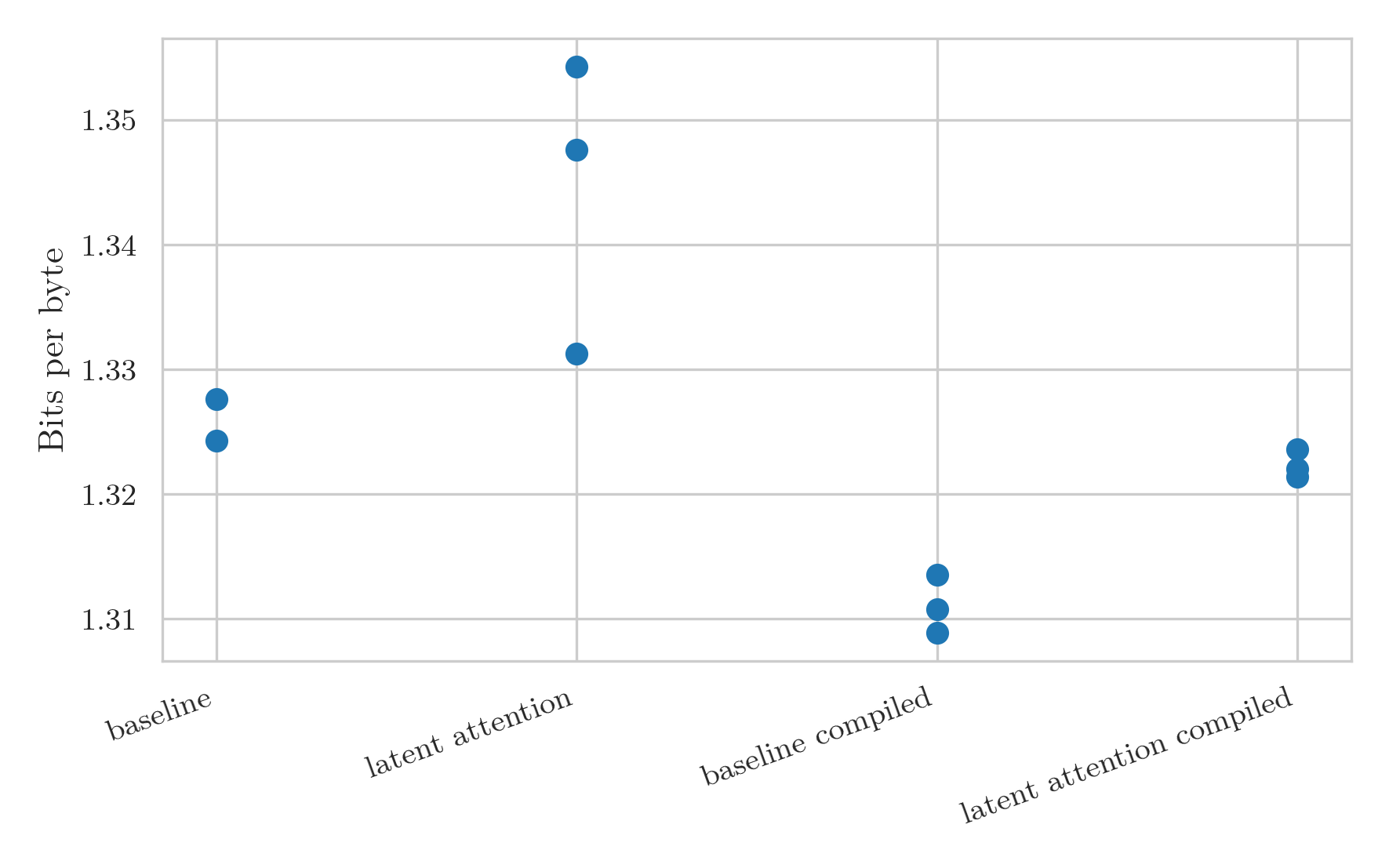
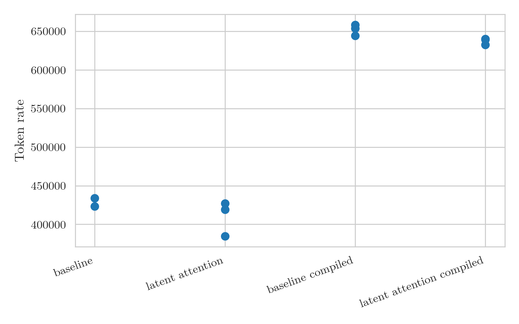 This was a great success. Not only is the throughput massively higher, but it is also much less noisy.
The increase in token rate leads to a distinct decrease in the BPB for the models:
This was a great success. Not only is the throughput massively higher, but it is also much less noisy.
The increase in token rate leads to a distinct decrease in the BPB for the models:
 The main problem with the compiled version is that the probes that calculate how many descent steps fit in 30 minutes are thrown off by the initial compilation.
I ran the projection sweep again, and adjusted the warmup steps to 200 and memory test steps to 100 to attempt to account for the compilation time.
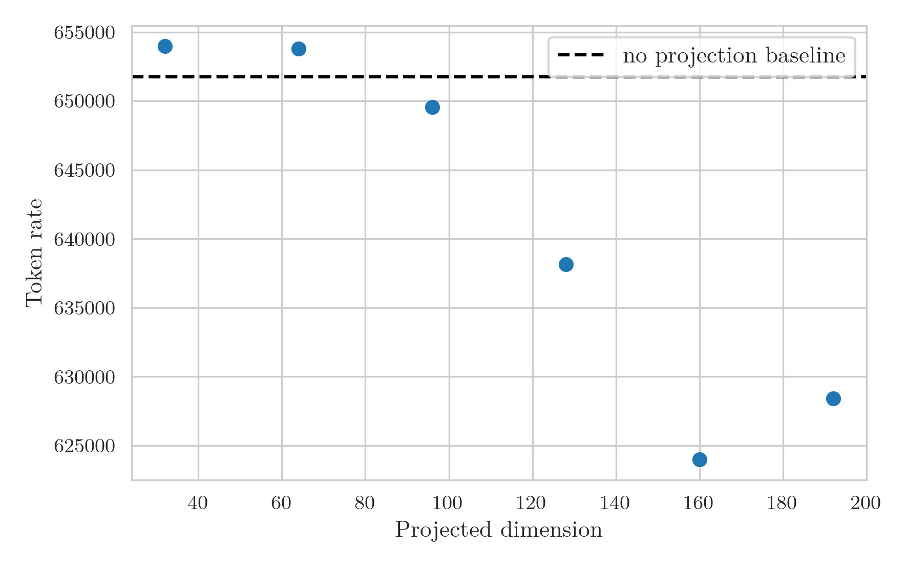
While the runs still didn’t go for the full anticipated 30 minutes, taking around 26 minutes instead, the results make a lot more sense than the previous graphs.
The token rate graph now shows a smooth decrease in rate as projection dimension increases, with a high bar from the baseline model likely stemming from the GPU overhead arising splitting the KV multiplication into two separate multiplications.
The main problem with the compiled version is that the probes that calculate how many descent steps fit in 30 minutes are thrown off by the initial compilation.
I ran the projection sweep again, and adjusted the warmup steps to 200 and memory test steps to 100 to attempt to account for the compilation time.
While the runs still didn’t go for the full anticipated 30 minutes, taking around 26 minutes instead, the results make a lot more sense than the previous graphs.
The token rate graph now shows a smooth decrease in rate as projection dimension increases, with a high bar from the baseline model likely stemming from the GPU overhead arising splitting the KV multiplication into two separate multiplications.
 The BPB graph is still a bit noisy at large projection dimensions:
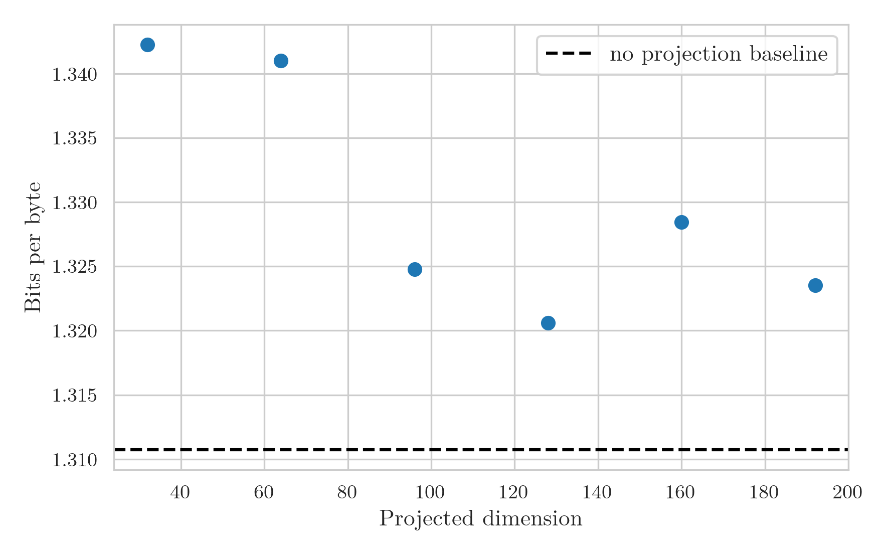 But I think shows a couple of things quite clearly.
Firstly, the expected pattern is now seen.
The BPB decreases as projection dimension increases due to the increased expressivity of the layer.
However, at a dimension of around 128, a minimum is achieved where above this the added cost restricts the number of tokens processed enough that the model starts to perform worse.
Secondly, the overhead from breaking up the matrix multiplication drowns out any performance gain from reduced FLOP and parameter counts, at least at this small scale.
This means that latent attention likely isn’t a viable method for increasing training performance, and should be used for its primary use case of increased KV caching efficiency.
But I think shows a couple of things quite clearly.
Firstly, the expected pattern is now seen.
The BPB decreases as projection dimension increases due to the increased expressivity of the layer.
However, at a dimension of around 128, a minimum is achieved where above this the added cost restricts the number of tokens processed enough that the model starts to perform worse.
Secondly, the overhead from breaking up the matrix multiplication drowns out any performance gain from reduced FLOP and parameter counts, at least at this small scale.
This means that latent attention likely isn’t a viable method for increasing training performance, and should be used for its primary use case of increased KV caching efficiency.
Final performance
The performance of the compiled baseline model and the best-performing latent attention model are found in the table below, averaged over two seeds each. I’ve decided to stop also testing on SimpleStories. The main purpose of this project is to have fun, and supporting two datasets was making me have less fun.
| Model | Bits per Byte |
|---|---|
| Compiled Baseline | 1.31 |
| Latent Attention | 1.32 |
Benchmark generations and training commits
Here are the generations from the standard prompts and the links to the specific commits used to train the models.
Compiled Baseline
Example Generations:
caitlin stood on the side of the house.
jayden had a jolly good time.
in japanese culture, women are often called "saturdaya" (the "saturdaya" or "saturdaya").
Latent Attention
Example Generations:
caitlin stood on the door.
jayden had a jolly good time.
in japanese culture, women are often called "survivals".